Data Science Projects

These Repository contains various Data Science projects I worked on for acadamic and self learning purpose. The projects are presented in IPython Notebooks using Jupyter Notebook as well as a python script file.

Projects

1. Predicting Probability of Credit Default (Logisitc Regression, Decision Tree and Random forest models)
2. Sentiment Analysis on Twitter data (Logistic Regression, Naïve Bayes and Support Vector Machine)
3. S&P 500 Stock Index Prediction (Multiple Linear Regression)
4. Data Cleaning and Preparation on Halloween Candy Survey data (Pandas, NumPy, Matplotlib)
5. Predicting antique watch prices in R using Linear Regression (Multiple Linear Regression)

Predicting Probability of Credit Default

I worked on a dataset found from the UCI Machine Learning Repository. The dataset contains information on default payments, demographic factors, credit data, history of payment, and bill statements of credit card clients from Taiwan for the time period of April 2005 to September 2005. I choose to analyze this dataset because of my curiosity in finding factors that contribute to defaults and finding signals that could indicate to defaults ahead of time that can help lenders decrease their loss. If defauly can be predicted accurately in advance, lenders could decrease the avaliable limit or possibly close the account and cut their loss short.

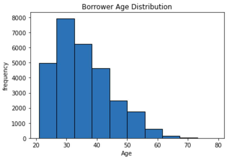
After reading the data into jupyter notebook and explored in details, my initial finding indicated the dataset had many irrelevant features I was able to drop. This dataset did not contain missing values, it did however had many values that were inconsistent. After doing some analysis comparing key features using comparasion operators, I was able to filter out the inconsistent data. For example in the Age column, I used the average age to replace some of the rows where the entered data was not consistent. After the initial cleaning steps I utilized the KBinsDiscretizer function to put the age groups into bins and encoded the nominal and ordinal features. I utilized the min max scaler function to scale others features.

Plotting Age Distribution

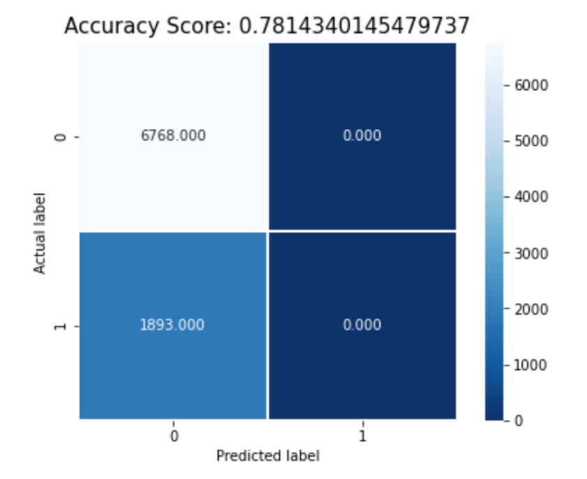
After preping my data for modeling by cleaning and scaling, I used three classfication models to predict and compare performance. I used Logisitc Regression, Decision Tree and Random forest models. I used the accuracy metric for performance evaluation. All three models performed nearly identical with an accuracy of 80% However the Decision Tree model performed a little better when using depth of 3. I learned the importance of hyperparameter tuning which helped increase the accuracy of Decision Tree from the initial result of 72% with defauly parameters to 82% accuracy.

Plotting Heatmap for Logistic Regression

Plotting Heatmap for Random Forest

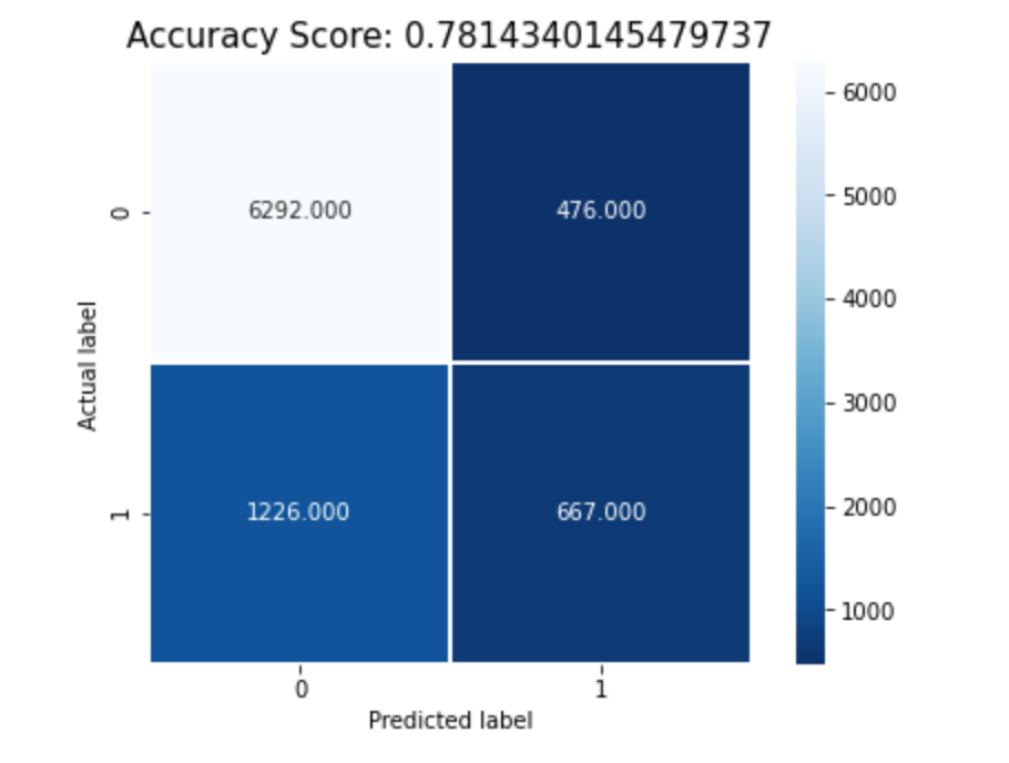
In conclusion although I was able to obtain 82% accuracy on all three models, more research can be completed to find any hidden signs that can direct us to the solution and avoid significant loss. I was able to see that some of the biggest factors were credit utilization, available balance, payment history, and possibly age. I believe that lenders can use this type of data and monitor all customers to cut down losses and increase profit margins.

Sentiment Analysis on Twitter data

Sentiment Analysis on data obtained from Twitter for the major US airlines: The objective of this task is to build a model that can accurately classify a social media tweets for the major US airlines as positive or negative based on the writers polarity. Arriving at a model that can predict and classify customers sentiment accurately can be beneficial for any sector and use it to improve services and products. It can also be used as a major input to busines models and help the company achieve higher revenue. One applications where sentiment analysis can be used is for decision making in a business by analyzing public opinion and developing new strategies. Sentiment analysis can also be used to gain advantage over the competitors.

In this project I explored with different models and utilized parameter optimization techniques to arrive at a model with the best accuracy. The models I explored with were Logistic Regression, Naïve Bayes and Support Vector Machine. The Pandas and Numpy libraries were utilized to clean and prepapre the data. The NLTK library and the Bag of Words approach were also used to transform and tokenize the words.

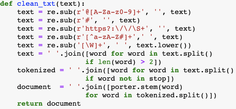
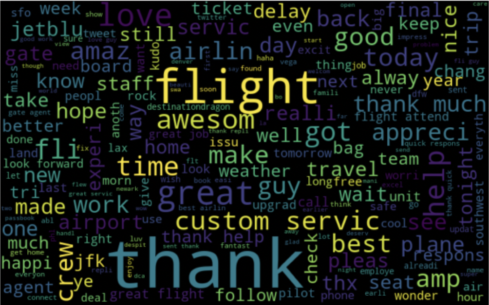
The first and the most important step in any Data Science project is data cleaning and data preprocessing. In order to achieve a high accuracy, cleaning our data is a vital step. During explanatory analysis I dropped unnecessary features. The three features used were Airline names, tweets and label. I utilized the Pandas and NumPy library’s for analysis and explanatory steps. The Regular Expression (RE) library was used to clean the text feature as well as the NLTK library to tokenize and stem the text. In order to arrive at high accuracy level the data we feed to the program needs to be clean. One of the approach I followed was to remove short words that have less than three characters. Even though the Stop words library was used to remove common words, it does not however remove every common words. Below is the function used to clean the data and some visualization with word cloud library.

Most frequently used words in Positive Sentiments

Most frequently used words in Negative Sentiments

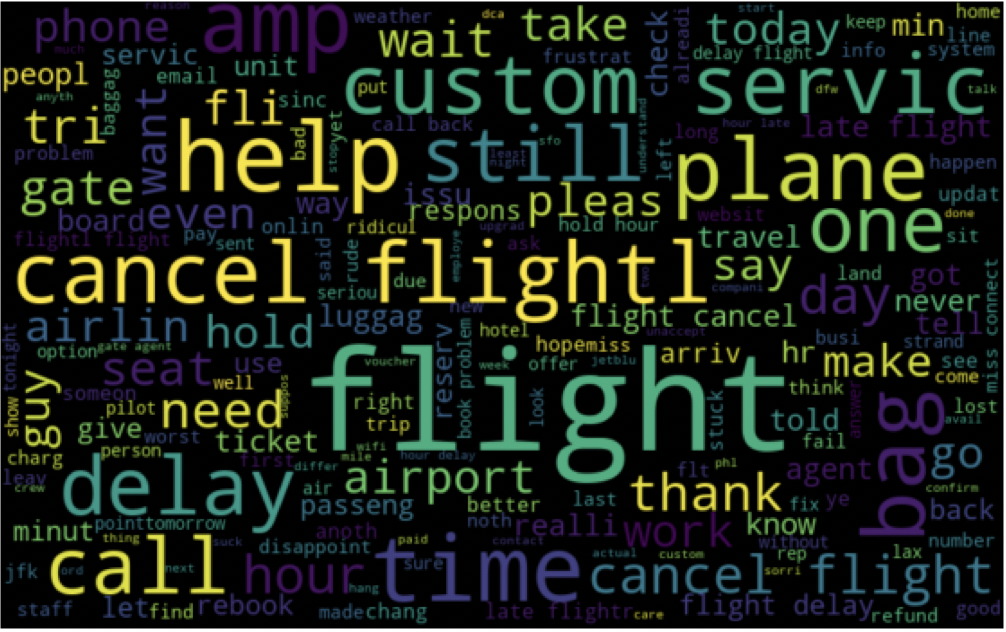
In conclusion, SVM gave us the best accuracy, However it is not an ideal approach to take in the real world because of the computational cost. Logistic Regression had similar result to SVM and it’s a better model to use. The Naïve Bayes model was lower in accuracy compared to the other models however I prefer to use the Naïve Bayes model due its simplicity and its flexibility to handle high dimensional feature. NLP is still rapidly growing and there is still much more work and research to be done in this field. I was able to obtain accuracy in the high 70’s with three targets and over 90% with two targets on every model I trained. However I believe there is more work I can do to improve my results particularly in the data cleaning and preprocessing steps.

S&P 500 Stock Index Prediction

Stock market Indexes are a powerful indicator of the global and country specific economies. Although there are many different types of Index avaliable to be utilized by investors, the three widely followed and used Indexes in the U.S. are the S&P 500, Dow Jones Industrial Average and Nasdaq Composite. The S&P 500 index is composed of the top 500 companies. These Indexes aggregate the prices of all stock together based on the weight it carries and allow investors to evaluate the market.

In this project, I used historical time series data on the price of the S&P 500 Index to make predictions about future prices. Each row in the data represents a daily record of the prices change for the Index starting in 2015 to 2020.

After fitting the linear regression model using 7 computed indicators, I was able to get MAE of 58.25 which is high considering our prices ranges from 2000 to 3626 but it is not a significantly large number. After expermenting by adding and removing indicators, with 5 indicators the MAE slightly dropped to 57.23 but not a significant change. I will try to compute and experment with more indicators that might give me a better insights into future prices of S&P 500 prices.

Data Cleaning and Preparation on Halloween Candy Survey data

The main objective for this project is to have an accurate, consistent and complete data from the Candy Hierarchy Survey dataset. There are many issues that needs to be fixed within the dataset in order to make the dataset ready for data analysis. We plan to work on removing some errors such as typos, inconsistent capitalization and mislabeled classes. Eventhough most of the surveys were multiple choice answers allowing the participants to pick thier answer, Some of the questions including the ones asking for the participants information were open questions allowing them to answer by typing their answers which lead to more Structural errors. We will work on those columns by filtering and fixing the common errors. There are also many missing data which needs to be fixed in order to have a complete data. We will also identify feature engineering opportunity if there are any.

While cleaning the data, we noticed several issues with missing data and inconsistent data. The “age” column contained strings values with participants who chose not to disclose their age. The “Country” column contained many typos, abbreviation and inconsistent entry. To solve these issues we were able to build a set that contained all common typos and different names and looped through the column to replace the errors with the correct value. Our primary objective was to do data analysis and answer some basic questions on U.S. and Canada. We removed all data that was not from these two countries.

From the box plot we can see the averge score among male, female and others are similar. However, the interquartile range for male is more narrow than female. Based on the graph, we can assume that female have a stronger sentiment about the taste of the candy. When the categories are less than 5, pie chart is useful to vizualize the distribution. As the gender distribution chart shows, there are 4 categories (Male, Female, Others and I would rather not say). From the chart we can easily see the proportion of male is more than 50%. However, if there are too many variables, a pie chart might make it harder to easily visualize and a bar plot might be a better option. To detect the popularities of 103 different types of candies we used a bar plot to describes the scores of each candy.

Predicting antique watch prices in R using Linear Regression

The objective of this project is to predict future prices of Antique watches using Multiple Linear Regression. The data used is from Mendenhall and Sincich (1993, page 173).The variables used in this model are “Age of the clock” as independent variable, “Number of individuals participating in the bidding” as the second independent variable and “selling price of the clock” as the dependent variable. The research questions are 1) To find if the ages of the clock and number of bidder variables predictive selling price of the clock accurately. 2) If they are predictive variables, how well do they predict it? I will be using regression analysis for multiple predictor variables to study the relationships between the variables.

Plotting Price Distribution

A multiple regression model was run to predict selling price of the clocks from number of bidders and age of the clock. These variables statistically significantly predicted the selling price.

Linear Regression Model Output

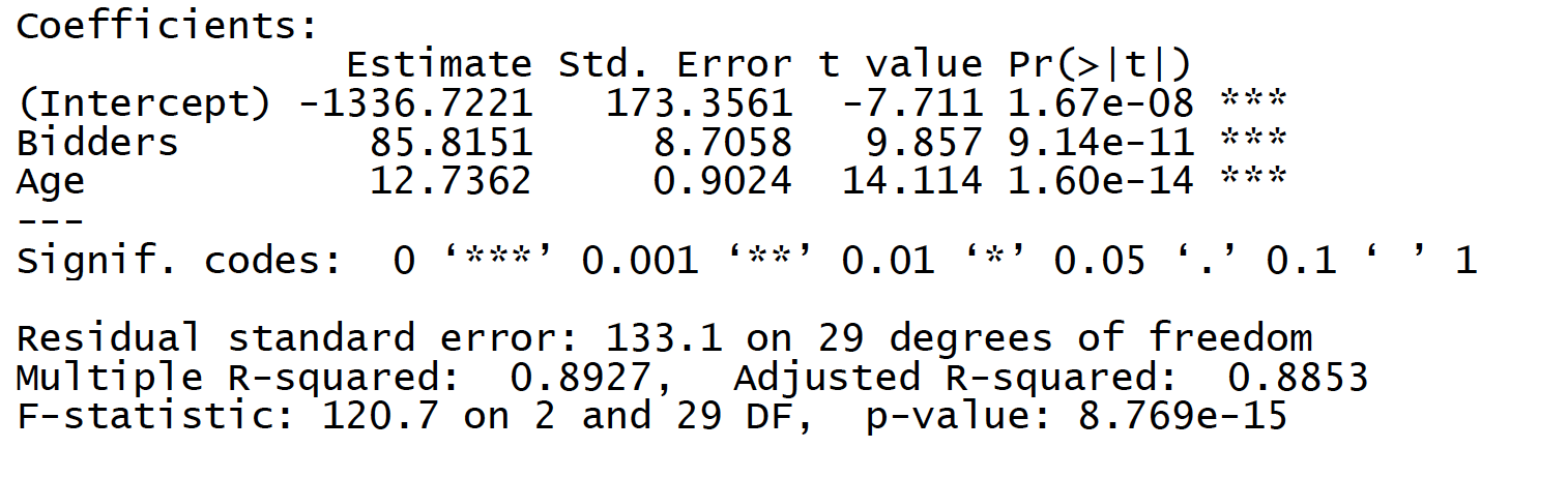
F(29) = 120.7, p < .0005, R2 = .893. The two variables added statistically significantly to the prediction, p < .05.

The regression equation is: 𝑌 = −1336.7221 + 85.8151(𝐵𝑖𝑑𝑑𝑒𝑟𝑠) + 12.7362(𝐴𝑔𝑒)

This equation means that for every bidder the predicted price will increase by 85.82 pounds sterling with a constant age. On the other hand, for every year added to the clock it will be an increase of 12.74 pounds sterling with a constant bidder. We can also notice that both the Multiple R-squared and the Adjusted R-squared are approximately 89% which shows how well the regression model explains the data.